SAO Guest Contribution

SAO Guest Contribution |
|
Alexander Knebe is a newly arrived postdoctoral fellow at the Centre for
Astrophysics and Supercomputing. He works on cosmological simulations of the
evolution of the Universe, and in this presentation he explains how such simulations
are being preformed using modern compuational techniques.
Alexander spent the last two years at Oxford Unviversity developing one of the few
adaptive grid-based codes for such tasks. He completed his PhD theis on "The
formation and evolution of galaxy clusters within the large scale structure of
the Universe" at Astrophyscial Institute Potsdam in Germany.
The Universe is expected to have started with a Big Bang in which -
or more precisely: shortly afterwards - tiny fluctuations were
imprinted into the radiation and matter density field (in the
otherwise homogeneous and isotropic Universe). To understand how the
Universe evolved from that early stage into what we observe today
(stars, galaxies, galaxy clusters, ...) one needs to follow the
non-linear evolution of those density fields using numerical methods.
So, the process of a cosmological simulation is actually twofold: one
first needs to generate some initial conditions according to the
structure formation model one likes to investigate, which are then used
as an input to the code itself. In all codes the evolution is
simulated by following the trajectories of particles under their
mutual gravity. And the law of gravity is simply just the Newtonian
force law
These particles are supposed to sample the matter density field as
accurately as possible and a cosmological simulation is nothing more
(and nothing less) than a simple and effective tool for investigating
the evolution of millions of particles. However, there are two
constraints on a cosmological simulation, (a) the correct initial
conditions and (b) the correct final particle distribution which ought
to agree with observations of the Universe as seen today. In
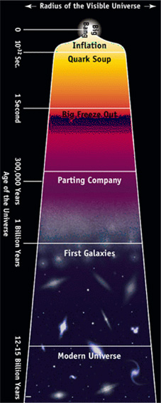
Fig. 1 you can find a rough sketch of the cosmic evolution
the Universe went through and simulations are trying to bridge the gap
between observations of the early Universe (i.e. anisotropies in the
Cosmic Microwave Background observed as early as 300000 years after
the Big Bang) and the modern Universe.
The first application of numerical simulations in astrophysics was the
simulation of star clusters [1] using as little as a couple of hundred
particles. During the 1970's more simulations of galaxy clustering
were performed using what is called PP (particle-particle)
methods [2] and finally in 1981 the first cosmological simulations
using more than 20000 particles appeared [3]. However, already those
simulations were able to make credible predictions and the problems
showing up in them remain unsolved even when using the latest high
resolution simulations, i.e., the steep rise of the density profile of
galaxies in the very central parts predicted by the simulations which is not matched by observation.
It is necessary to use as many particles as possible because the idea
always is that the particles are sampling the density of the Universe
rather than being individuals. This is different to using numerical
simulations for modelling the formation of globular clusters where
each particle represents a single star. In a cosmological simulations
the particles are not to be confused with galaxies, stars, or
whatever. They are more to be understood as sampling points of a
fluid/density field that moves under its own gravity. But the problem
is that the more particles used, the more computer time a
simulation consumes. And even with the largest supercomputers nowadays
it is only possible to use some million particles if we want to
retrieve results in a reasonable time (say, couple of weeks). And until
now the methods for simulating millions of gravitationally interacting
particles have been continiously refined to allow for more and more
particles to be used while simultaneously resolving finer and finer
structures. These simulations can resolve the orbits of dwarfs
galaxies (
In this contribution I would like to focus on various numerical
techniques, their advantages and their shortcomings when being
compared with each other. I need to stress that all those simulations
are based on the assumption that the Universe mainly consists of Dark
Matter that only interacts via gravitation. Baryonic matter, which
only accounts for about 10% of the total mass of the Universe, is
completely neglected in these simulations. Only nowadays the methods
and the computer technology have become as sophisticated as to allow
for hydrodynamical processes (i.e. gas dynamics) to be included in
such time consuming calculations, but the field is still in its
infancy.
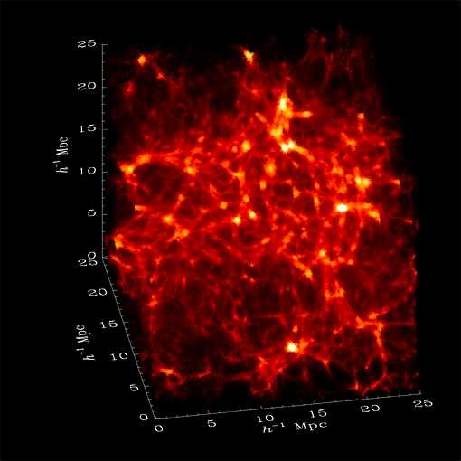
Finally, have a look at Fig. 2 to get an idea of what it looks
like to simulate the Universe in a computer.
with the correct choice for the force
As already mentioned in the Introduction, each particle feels a force
that is given by the Newtonian gravity law:
Because we need to take into account the forces from all particles
other than particle
However, Eq. (2) is just the special case where we are dealing
with point-like masses. But the actual idea is to use the particles as
sampling points for the density. Therefore the correct equation to use
is not Newton's force law Eq. (2), but the generalisation of it
- called Poisson's equation:
One can see that this equation involves the density
Once we know the potential,
Anyway, their are two different techniques being used for
cosmological simulations. The one is based on Eq. (2) and the
other on Eq. (3):
which will be explained in more detail later on.
Moreover, the size of the simulation box also defines the mass
resolution of the simulation. We are only using a certain number of
particles within a well defined region of the Universe (the box). And
as the denisty of the Universe is given by the cosmological model
under investigation, we can calculate the mass of a single
particle. This mass determines the mass resolution of that
specific simulation. For instance, if we model the evolution of about
2 million particles in a (25
Because we are interested in deriving the forces at every single
particle position, the PP method scales like
One publically available Tree code is called GADGET (Galaxies
with Dark Matter and Gas intEracT)
written by one of my colleagues Volker Springel [5]. Feel free to
download it from the following web page and have a play with it: http://www.mpa-garching.mpg.de/gadget/
The scale defined by the parameter
In this scheme most of the time is also spent at point 2 and there are
various methods for solving Poisson's equation.
Introduction
The purpose of a cosmological simulation is to model the growth of
structures in the Universe and have a long history and numerous
applications. These simulations play a very significant role in
cosmology because they are the one and only 'experiment' to verify
theories of the origin and evolution of the Universe.
![]() where
where ![]() (the 'r with two dots' is just another way of writing the second derivative of r, ie. d2r/dt2, which is just the acceleration).
(the 'r with two dots' is just another way of writing the second derivative of r, ie. d2r/dt2, which is just the acceleration).
![]()
![]() ) within galactic haloes
(
) within galactic haloes
(
![]()
![]() ) in cosmological volumes of
the order (30
) in cosmological volumes of
the order (30![]() )
)![]() [4].
[4].
Newtonian Gravity
The whole idea is to use Newton's second law
![]() . And most of the
computational time during a numerical simulation of the Universe is
actually spent on deriving the forces at every single particle
position.
. And most of the
computational time during a numerical simulation of the Universe is
actually spent on deriving the forces at every single particle
position.
![]() the force on this particular particle
the force on this particular particle
![]() is the sum (
is the sum (![]() ) of all the forces from the other
particles (as given by Eq. (2)).
) of all the forces from the other
particles (as given by Eq. (2)).
![]() and it can
be easily proved that the assumption of dealing with point-like masses
leads to exactly Eq. (2) for the force
and it can
be easily proved that the assumption of dealing with point-like masses
leads to exactly Eq. (2) for the force ![]() . The new
quantity
. The new
quantity ![]() introduced in Eq. (3) is called the
potential and in the theory of classical mechanics it is a
more convenient way of describing gravity to use
introduced in Eq. (3) is called the
potential and in the theory of classical mechanics it is a
more convenient way of describing gravity to use ![]() rather than
the force vector
rather than
the force vector ![]() .
.
![]() we can readily calculate the force
at each particle location which is crucial for integrating the
equations of motions Eq. (1). The proper way of doing so is going
to be outlined later on in the Section on Newtonian Dynamics.
we can readily calculate the force
at each particle location which is crucial for integrating the
equations of motions Eq. (1). The proper way of doing so is going
to be outlined later on in the Section on Newtonian Dynamics.
1. direct particle-particle summation as given by Eq. (2)
![]() Tree Codes (or PP method)
Tree Codes (or PP method)2. numerical integration of Eq. (3) on a grid
![]() Particle-Mesh Codes
Particle-Mesh Codes
Mass Resolution
I still need to mention that a cosmological simulation in practice
only simulates a certain part of the Universe. This is what people
refer to as the simulation box or computational
box. However, to account for the fact the Universe actually is
indefinite one uses periodic boundary conditions: particles leaving
the box on the one side are immediately entering the box again on the
other side. This is sketched in Fig. 3 which indicates how
a particle leaving the right side of the computational box enters
again on the left hand side.
![]() )
)![]() box within a
box within a ![]() CDM model
(
CDM model
(
![]() ), each particle weighs about
), each particle weighs about
![]()
![]() . So, we won't be able to resolve dwarf galaxies in that
particular cosmological simulation (since
. So, we won't be able to resolve dwarf galaxies in that
particular cosmological simulation (since
![]()
![]() ).
).
Tree Codes - The Forces
The PP (particle-particle) method upon which Tree
codes are based assumes to deal with point-like masses and therefore
Eq. (2) is applicable. This is also why this technique is
called PP: it uses the direct particle-particle summation to calculate
the forces.
![]() : if we double the
number of particles it takes four times as much time to actually run
the simulation. Therefore this PP method is not feasible for a
sufficient number of particles, not even on the largest supercomputers
available nowadays ! One needs to come up with a more sophisticated
treatment decreasing the need for computer time, and one way of
achieving this is to organize the particles in a tree-like
structure: if particles are located ''far away'' from the actual
particle at which position we intend to calculate the force, these
particles can be lumped together as a single but more massive particle
at the mean distance (cf. Fig. 4). This decreases the number of
calculations dramatically, bringing such codes back into the field of
competition with other methods.
: if we double the
number of particles it takes four times as much time to actually run
the simulation. Therefore this PP method is not feasible for a
sufficient number of particles, not even on the largest supercomputers
available nowadays ! One needs to come up with a more sophisticated
treatment decreasing the need for computer time, and one way of
achieving this is to organize the particles in a tree-like
structure: if particles are located ''far away'' from the actual
particle at which position we intend to calculate the force, these
particles can be lumped together as a single but more massive particle
at the mean distance (cf. Fig. 4). This decreases the number of
calculations dramatically, bringing such codes back into the field of
competition with other methods.
Tree Codes - The Force Resolution
We need to (manually) set a limit on the minimal allowed spatial
separation between two particles for which we can actually calculate
the forces. This is because of the singularity arising from the
![]() force law in Eq. (2) which can be avoided by
introducing a (fixed) scale
force law in Eq. (2) which can be avoided by
introducing a (fixed) scale ![]() . This parameter determines the
smallest possible separation for two individual particles:
. This parameter determines the
smallest possible separation for two individual particles:
![]() is usually called the
softening parameter or the force resolution of a numerical
simulation run by a code which uses a PP summation.
is usually called the
softening parameter or the force resolution of a numerical
simulation run by a code which uses a PP summation.
Particle-Mesh Codes
Another way of deriving the forces is to use Poisson's
equation (3) and to numerically integrate it. This
approach is closer to the idea of a cosmological simulation which
intends to follow the evoution of the density rather than the
interaction of individual particles. But this method requires the
introduction of a grid on which we can define the density and also
solve Eq. (3) numerically. The grid is usually a regular one
with
![]() cells where each cell is identified by the
triple
cells where each cell is identified by the
triple ![]() with
with
![]() and
and ![]() (i.e., each of i, j and k run from 0 to L).
The itinerary for calculating the force at particle position
(i.e., each of i, j and k run from 0 to L).
The itinerary for calculating the force at particle position
![]() due to the denisty field of all particles looks
exactly like this:
due to the denisty field of all particles looks
exactly like this:
![]()
![]()
![]()
![]()
![]()
![]()
![]() back to particle positions
back to particle positions
![]()
Particle Mesh Codes - The Forces
I do not want to go into the details of how to numerically solve a
(partial) diffetential equation. The only thing that needs to be
mentioned is that most people use Fourier transformations. On the
largest supercomputers in the world there are software libraries
available which include the fastest routines for Fourier
transformations one can imagine. To actually benchmark supercomputers
this is the recognized procedure: the faster the Fourier transform the
better the computer. So, most supercomputer manufacturers (i.e. Cray, SGI,
IBM, ...) are working extremely hard on selling the world's fastet
Fourier transformations along with their machines. And this is why
this technique is adopted for solving Poisson's equation as needed in
cosmological simulations. However, there are other methods and one of
the publically available PM (Particle-Mesh) codes that uses a
different integration scheme was written by myself [6]. The code
can be downloaded along with exhaustive documentations and some
sample cosmological simulations at the following web address:http://www-thphys.physics.ox.ac.uk/users/MLAPM/
Particle Mesh Codes - The Force Resolution
The problem with the PM method is the lack of spatial resolution below
two grid spacings. Whereas in Tree codes one needs to manually fix the
problem of the singularity in Eq. (2) for close encounters of
particles by introducing the scale ![]() (cf. Eq. (4)), in
PM we are dealing with sort of the opposite. As gravity tends to clump
things together, the particles flow from low density regions into high
density regions amplifying primordial density fluctuations. This
leads to an excess of particles in certain cells whereas other cells
are becoming more and more empty. The PM method can be understood as
smoothing the density field (as defined by the particle positions) on
a scale determined by the spacing of the grid. Hence particles that
are closer than about two cells spacings do not interact according to
Eq. (3) with each other. We are left with the situation where we
can not resolve structure formation on scales smaller than the cell
spacing of the grid !
(cf. Eq. (4)), in
PM we are dealing with sort of the opposite. As gravity tends to clump
things together, the particles flow from low density regions into high
density regions amplifying primordial density fluctuations. This
leads to an excess of particles in certain cells whereas other cells
are becoming more and more empty. The PM method can be understood as
smoothing the density field (as defined by the particle positions) on
a scale determined by the spacing of the grid. Hence particles that
are closer than about two cells spacings do not interact according to
Eq. (3) with each other. We are left with the situation where we
can not resolve structure formation on scales smaller than the cell
spacing of the grid !
This is the major problem for PM simulations and the most obvious way to overcome this is to introduce finer grids in such regions. However, these grids needs to freely adapt to the actual particle distribution at all times and hence programming such an adaptive PM method is a very demanding task. Therefore not many research groups took that avenue and there are only a handful of such codes ([6],[7],[8]). One of them (and the only one to be publically available) is our very own code MLAPM (Multi-Level-Adaptive-Particle-Mesh) already mentioned.
You can get an idea of the nested grid structure for a radial (two-dimensional) particle distribution with sucessively more and more particles close to the centre in Fig. 5. The upper panel shows the particle positions whereas in the lower panel the adaptive grid structure for solving Poisson's equation is presented.
Of course there are other ways to increase the force resolution
locally and most of my colleagues are using what is called a P![]() M
code: a combination of PP and PM methods. Here the force as given by
the plain PM calculation is augmented by a direct summation over all
neighboring particles within the surrounding cells. This gives
accurate forces down to the scale provided by the softening parameter
M
code: a combination of PP and PM methods. Here the force as given by
the plain PM calculation is augmented by a direct summation over all
neighboring particles within the surrounding cells. This gives
accurate forces down to the scale provided by the softening parameter
![]() again.
again.
In my opinion the problem with Tree as well as with P![]() M codes lies
in the possibility of close encounters of two (or more) particles.
The formula for the force then becomes singular, because the
denominator reaches zero. This problem is fixed by the introduction of
a general scale
M codes lies
in the possibility of close encounters of two (or more) particles.
The formula for the force then becomes singular, because the
denominator reaches zero. This problem is fixed by the introduction of
a general scale ![]() (cf. Eq. (4)). When two
particles approach too closely they then undergo a huge acceleration
and the time step for integrating the equations of motion (time
stepping is going to be discussed in the following Section) might be
too small to account for that. Hence they bounce off each other
violating the conservation of energy (this effect is called
two-body scattering). Moreover, the softening applies to all
particles whether they are in a high denity region or a low density
region. If we want to resolve structures on kpc-scales in a simulation
box with sidelength a couple of Mpc's we need to do so from the very
start of the simulation and at every spatial location within
that box. But studies have shown that the force resolution should not
be better than the local (!) interparticle separation
([6],[10],[11]). Codes incorporating a PP direct summation are
therefore suffering from a force resolution that is spatially fixed.
Low density regions are over-resolved in these codes (which is a waste
of computer time as well as leading to artificial effects such as two-body
scattering) and high density regions might be affected by two-body collisions.
(cf. Eq. (4)). When two
particles approach too closely they then undergo a huge acceleration
and the time step for integrating the equations of motion (time
stepping is going to be discussed in the following Section) might be
too small to account for that. Hence they bounce off each other
violating the conservation of energy (this effect is called
two-body scattering). Moreover, the softening applies to all
particles whether they are in a high denity region or a low density
region. If we want to resolve structures on kpc-scales in a simulation
box with sidelength a couple of Mpc's we need to do so from the very
start of the simulation and at every spatial location within
that box. But studies have shown that the force resolution should not
be better than the local (!) interparticle separation
([6],[10],[11]). Codes incorporating a PP direct summation are
therefore suffering from a force resolution that is spatially fixed.
Low density regions are over-resolved in these codes (which is a waste
of computer time as well as leading to artificial effects such as two-body
scattering) and high density regions might be affected by two-body collisions.
The introduction of refined grids in PM methods on the other hand
guarantees to adapt the force resolution to the actual problem at all
times. If we start out with a grid where the number of grid cells ![]() per dimension is chosen so that two cell spacings agree with the
interparticle separation, we are doing fine. And as soon as particles
gather together in certain cells because of the attractive character
of gravitation, we split those cells in a manner such that the newly
created cells also have a spacing that agrees with the (local)
interparticle separation. This procedure is tuned to never ever
resolve better than the (local) mean separation length of particles
whether the particles are in high or in low density regions.
per dimension is chosen so that two cell spacings agree with the
interparticle separation, we are doing fine. And as soon as particles
gather together in certain cells because of the attractive character
of gravitation, we split those cells in a manner such that the newly
created cells also have a spacing that agrees with the (local)
interparticle separation. This procedure is tuned to never ever
resolve better than the (local) mean separation length of particles
whether the particles are in high or in low density regions.
Anyway, some Tree codes (i.e. GADGET) already take care of problems like the two-body scattering by adapting the time stepping scheme to the local acceleration and hence those authors might claim there is no problem with it at all. Therefore I need to stress that above statements are my personal point of view and this topic is still under hot debate as one needs to make absolutely sure that cosmological simulations are free of numerical artifacts !
Last but not least I need to mention the way of updating the positions and velocities of the particles. We are only dealing with Newtonian dynamics and therefore the equation to integrate is simply:
However, the Universe is expanding and it is far more convenient to
re-write this equation using what is called comoving
coordinates. This is a transformation to a non-inertial (accelerating) frame, but it
nevertheless simplifies things. Let us introduce the comoving variable
![]() :
:
where ![]() is the cosmic expansion factor. Actually calculating
is the cosmic expansion factor. Actually calculating
![]() is quite a complicated task because this involves
General Relativity. When Einstein wrote down his equations
describing gravity, people soon realized from the solutions to those
equations that the Universe needs to either expand or collapse (the
steady-state Universe was not covered by his orginal equations and was
only possible by introducing something like a negative gravitational
push). And to calculate the rate of expansion of the Universe
is quite a complicated task because this involves
General Relativity. When Einstein wrote down his equations
describing gravity, people soon realized from the solutions to those
equations that the Universe needs to either expand or collapse (the
steady-state Universe was not covered by his orginal equations and was
only possible by introducing something like a negative gravitational
push). And to calculate the rate of expansion of the Universe ![]() one needs to fully solve Einstein's General Relativity equations under
certain assumptions (homogeneity and isotropy). However, this
calculation is performed during the course of a cosmological
simulation and does not consume any of the computational time at all
-- it is an easy task once properly programmed.
one needs to fully solve Einstein's General Relativity equations under
certain assumptions (homogeneity and isotropy). However, this
calculation is performed during the course of a cosmological
simulation and does not consume any of the computational time at all
-- it is an easy task once properly programmed.
To time-step a cosmological simulation we need to have the
correct initial conditions with the particle positions and velocities
given in comoving coordinates at a specific time ![]() .
This system is then evolved forward in time until we reach todays time
.
This system is then evolved forward in time until we reach todays time
![]() where
where ![]() obviously depends on the
cosmological model. The 'gap' between
obviously depends on the
cosmological model. The 'gap' between ![]() and
and ![]() (cf. Fig. 1) is covered by a series of steps
(cf. Fig. 1) is covered by a series of steps ![]() which I already refered to as being the time step of the
simulation (cf. discussion of Tree vs. Particle Mesh). Early
cosmological codes (i.e. AP
which I already refered to as being the time step of the
simulation (cf. discussion of Tree vs. Particle Mesh). Early
cosmological codes (i.e. AP![]() M) use a fixed time step
M) use a fixed time step ![]() =const. whereas modern codes (i.e. GADGET and MLAPM) also adapt the
time step to the actual problem during the course of the simulation. I
have to admit that the Tree code GADGET uses a criterion that is based
on the local acceleration to match the integration of the equations of
motion (Eq. (5) combined with Eq. (6)) to the desired
needs for each individual particle. MLAPM only divides the global
time step set by the user for the first grid by successive factors of
two on the adaptively placed refinements. In any case, particles in
high density regions are updated more frequently leading to better
accuracy in the time evolution of the simulation.
=const. whereas modern codes (i.e. GADGET and MLAPM) also adapt the
time step to the actual problem during the course of the simulation. I
have to admit that the Tree code GADGET uses a criterion that is based
on the local acceleration to match the integration of the equations of
motion (Eq. (5) combined with Eq. (6)) to the desired
needs for each individual particle. MLAPM only divides the global
time step set by the user for the first grid by successive factors of
two on the adaptively placed refinements. In any case, particles in
high density regions are updated more frequently leading to better
accuracy in the time evolution of the simulation.
I haven't covered anything like setting up the initial conditions for a specific cosmological model yet, nor was there any comment on how to actually analyse a simulation. This again would go beyond the idea of this contribution, but feel free to either browse astrophysical journals as Monthly Notices of the Royal Astronomical Society, MNRAS or Astrophysical Journal, ApJ for it or to contact me directly via email (aknebe@astro.swin.edu.au).
| [1] Aarseth S.J., MNRAS 126, 223 (1963) |
| [2] Peebles P.J.E., Astron. J. 75, 13 (1970) |
| [3] Efstathiou G., Eastwood J.W., MNRAS 194, 505 (1981) |
| [4] Ghigna S., Moore B., Governato F., Lake G., Quinn T., Stadel, J., ApJ 544, 616 (2000) |
| [5] Springel V., Yoshida N., White S.D.M., NewA6512001 |
| [6] Knebe A., Green A., Binney J.J., MNRAS 325, 845 (2001) |
| [7] Kravtsov A.V., Klypin A.A., Khokhlov A.M., ApJ 111, 73 (1997) |
| [8] Norman M.L., Bryan G.L., in Numerical Astrophysics, |
| eds. S.Miyama, K.Tomisaka,T.Hanawa (Boston:Kluwer), 1998 |
| [9] Couchman H.M.P., ApJ 368, 23 (1991) |
| [10] Binney J., Knebe A., astro-ph/0105183 |
| [11] Hamana T., Yoshida N., Suto Y., astro-ph/0111158 |
| [12] Peebles P.J.E., The large-scale structure of the Universe, Princeton University Press, 1980 |
| [13] Bertschinger E., Ann. Rev. A & A 36, 599 (1998) |
| [14] Hockney R.W., Eastwood J.W., Computer Simulations Using Particles, Bristol: Adam Hilger (1988) |