Visualization Stages - Technical Notes

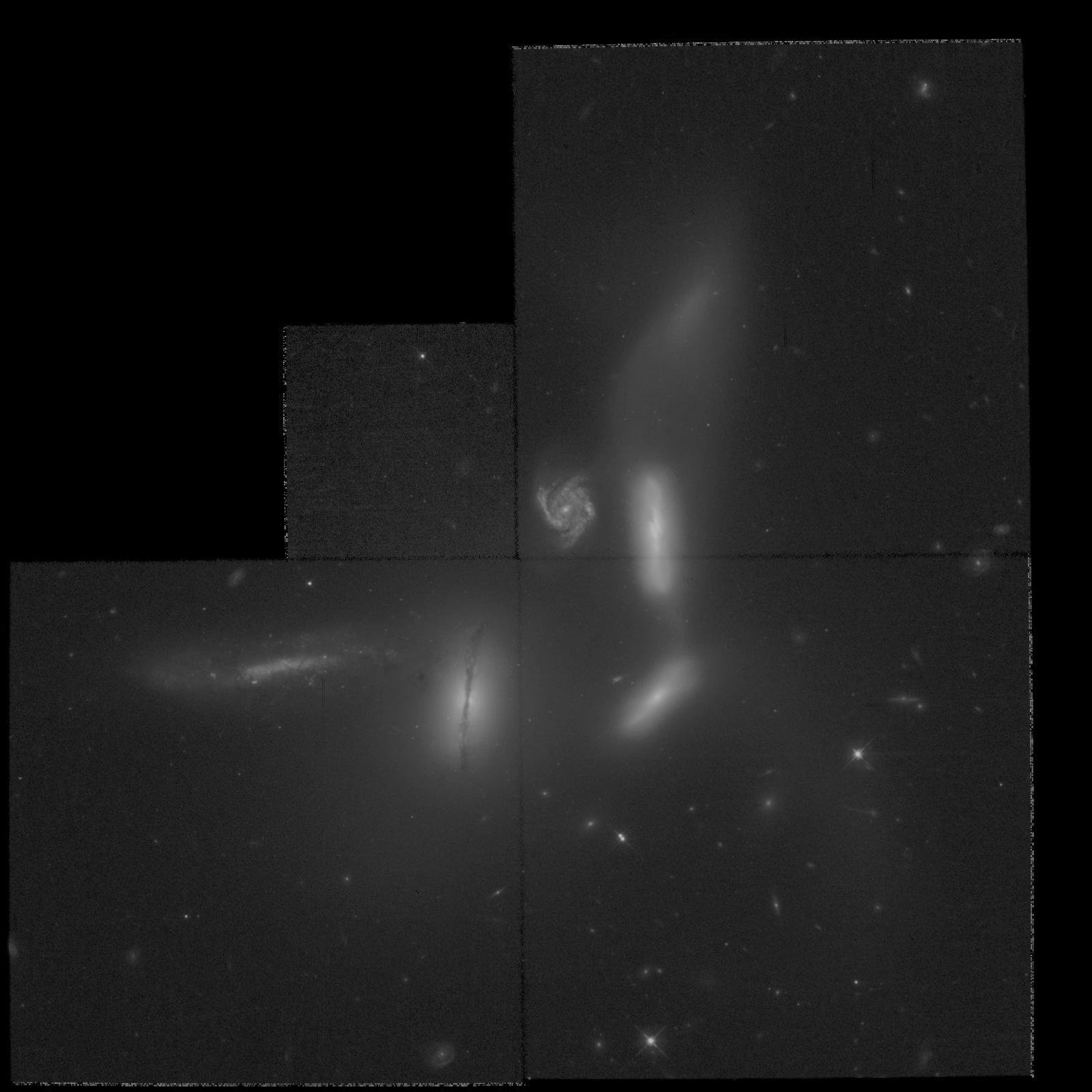
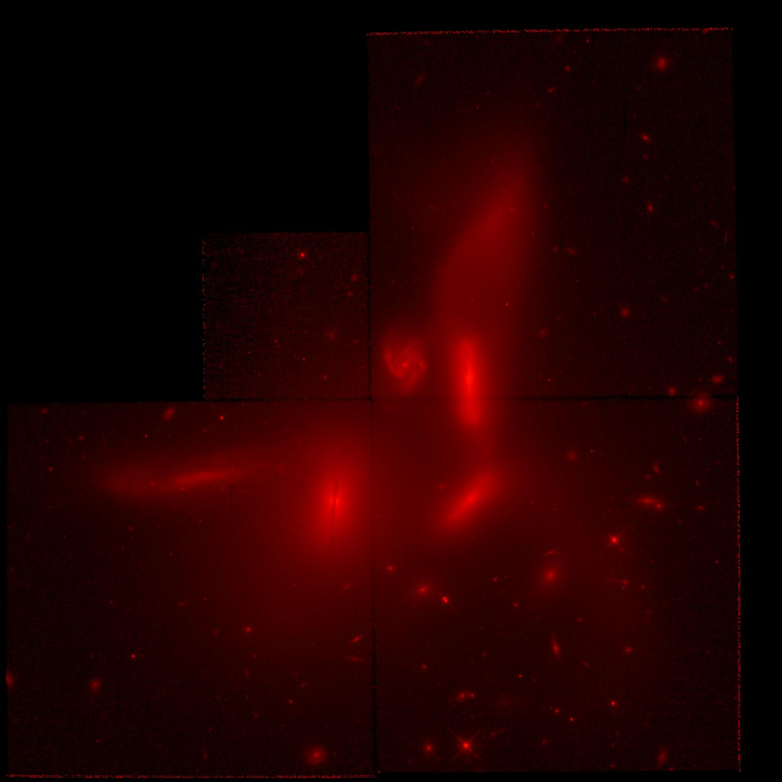
Stage 1: The stretch:

Software	comments
IDL	This costs money and you have to do your own coding.
RGBSUN in IRAF	Requires trial and error for the thresholds and you can only combine 3 filters.
kvis	Free in the Karma suite. http://www.atnf.csiro.au/computing/software/karma/. This let's you select thresholds in real time via histograms. As well as linear and log scaling, does square root which is good for nebulae. It has additional algorithms in its pseudo-colour option (best is greyscale3). Also it exports your scaled image to Portable Pixel Map format which is accepted by all many packages.

In Karma, using kvis, you can reduce an image by loading a fits file with the filter option turned on. Select the number of pixels to "skip" (which is actually "add together"). Adjust your image and then export this to a new ppm image. If you are using another package for stretching the intensities, then a good format to save the file as is tiff format, if it is available.

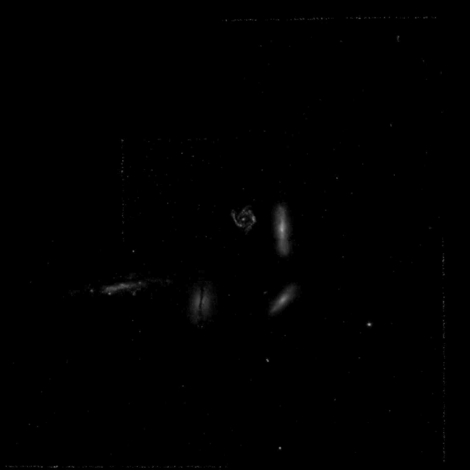
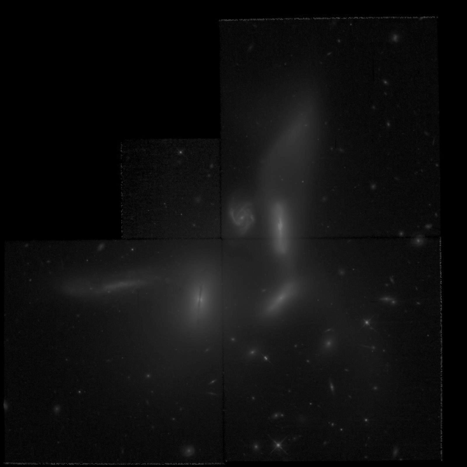
Original Image	Stretched Image

Stage 2: Layering and Assigning Colours:

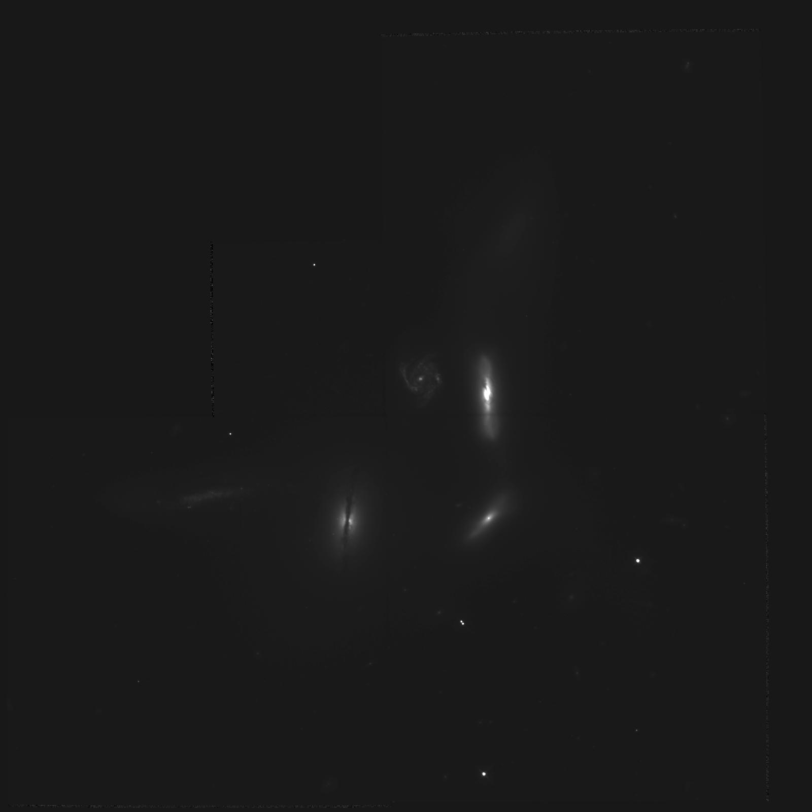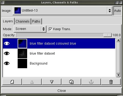
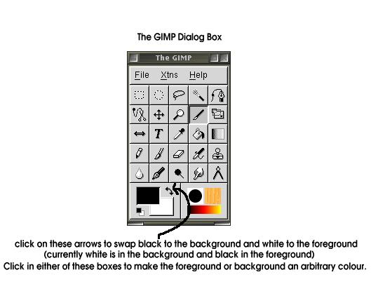
Next pump your output from the Stage 1 (above) into a manipulation package such as GIMP or PhotoShop. Your work is done in "layers" (rather than in colour channels) -- so open up the Layers Dialog Box in your manipulation package. Create a layer for each Stage 1 black and white dataset image. About "layers" in general:

• Layers allows one to assign any colour, not just a primary colour, to an image. (See an example at http://www.ras.ucalgary.ca/CGPS/press/shell/)
• In order to see all the images in your stack of layers, "screen" is a good algorithm. This mode is set, using a menu on the Layer Dialog Box, for each individual layer. A layer with this mode is like a transparency or positive slide, allowing light from the image below it to shine through it.
• Each layer is individually adjusted so a noisey image, say from one filter's dataset, can be suppressed without affecting the other images. To suppress noise you can apply a gaussian filter to the pixels, smoothing them out.

• Click your right mouse button in the image window in order to access the task menus.

1. In Gimp open up an image.
2. Then open up a new image with the background set to black by selecting the foreground or background as appropriate. Ensure the Layers, Channels, Paths dialog box is open.
3. On your original image, right clicking to get the menu options, find Edit --> Copy visible. On the new image, Edit --> Paste. This will put the B&W image into a layer.
4. In the Layers dialog box, click on the words "floating section" and give the layer a name. This will also change layer into something you can edit.
5. Set the mode algorithm, in the Layers, Channels, Paths dialog box. IMPORTANT: in order to see each of the layers, not just the top one, you need to select a relevant mode. "screen" is a good algorithm for combining images; it is set on each of the layers (or you won't see the one underneath).
6. Repeat for other images.
7. Save this layered image as an ".xcf" format file.

Then for each layer you assign a colour. This you do using the Levels tool.

1. Click on the name of a layer in the Layers, Channels, Paths dialog box so that it is blue which means active.
2. Go get the levels tool. [Image --> Colors --> Levels tool]
3. Change the top menu in the levels tool from value to a colour and adjust the OUTPUT levels to get your requested colour. (For example, if you want your layer to be green, then change the menu to Red and drag the right slider in the output levels to zero... repeat this for Blue... your layer should now be Green).
4. Repeat for each layer.
5. Save this as a .xcf format file.
6. Adjust values and colours until you are happy with the results. For example, if one filter image is particularly noisy (textured), this can be reduced by applying to that layer a gaussian filter with the width of the noise (e.g. a few pixels).
7. Save changes as a .xcf format file.

Some advise: Make copies of your B&W layers and work on those so you don't have to insert images again. Sometimes turn off the other layers (by clicking on the eye icon) to check your colours.

This is very iterative. Enjoy!

Other options: Some imagemakers work on one RGB image (i.e. 3 filters) and then layer in other filters at this stage. For an example, at http://heritage.stsci.edu/public/apr1/h301filt.html is an RGB image from 3 filters with other filters layered on top.

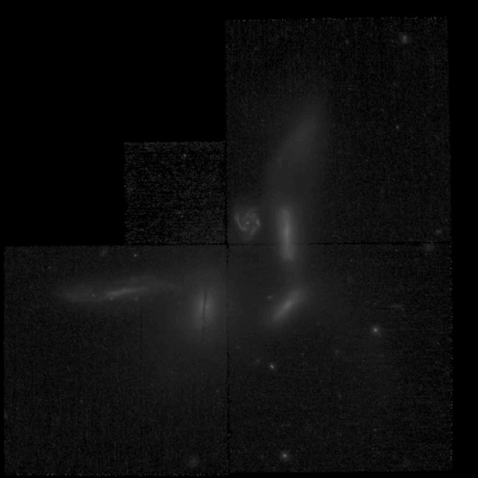
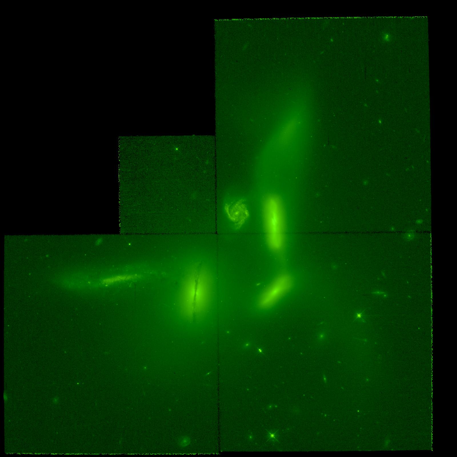
Filter	Black and White Stretch Image	Colour Assigned to Image
Ultraviolet
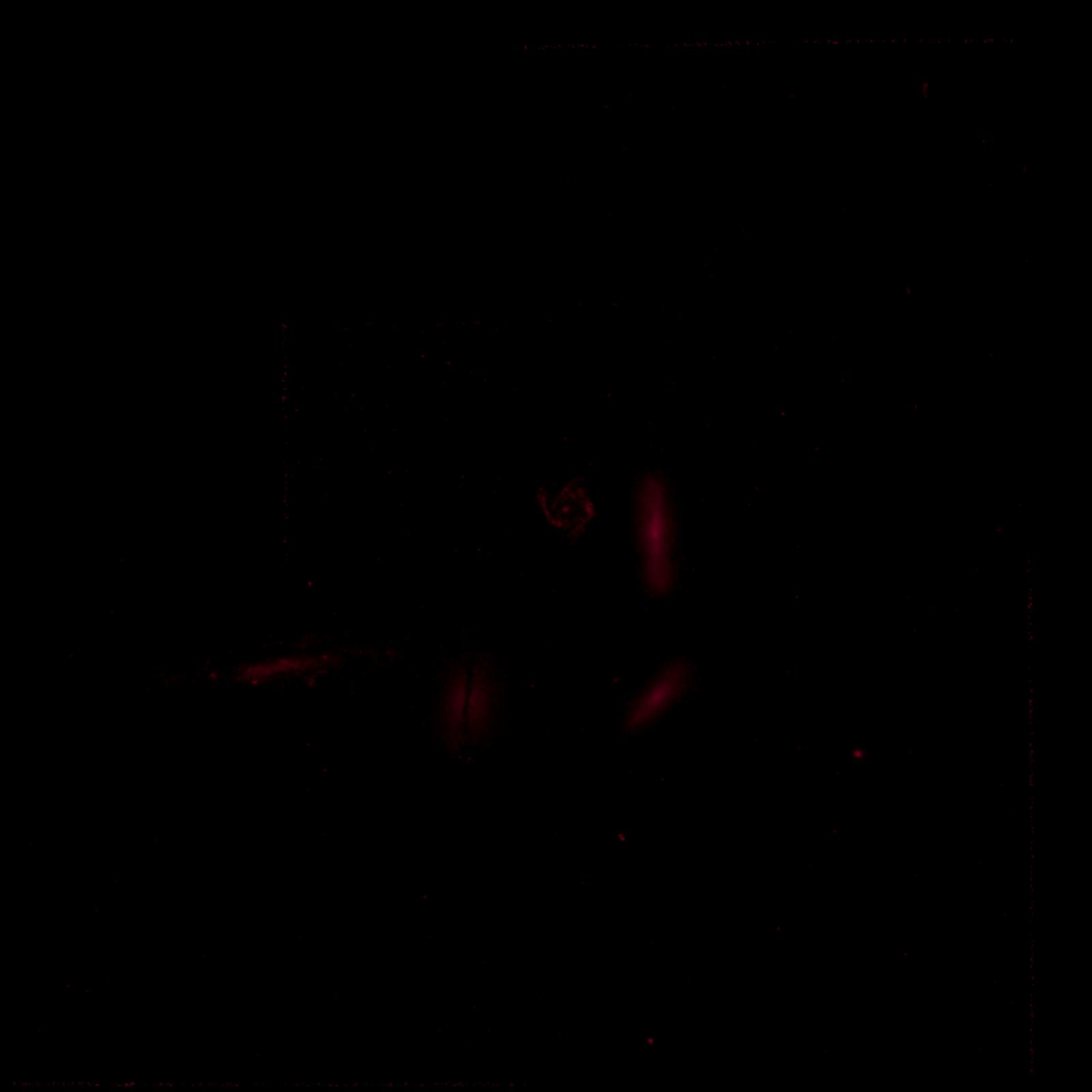Blue
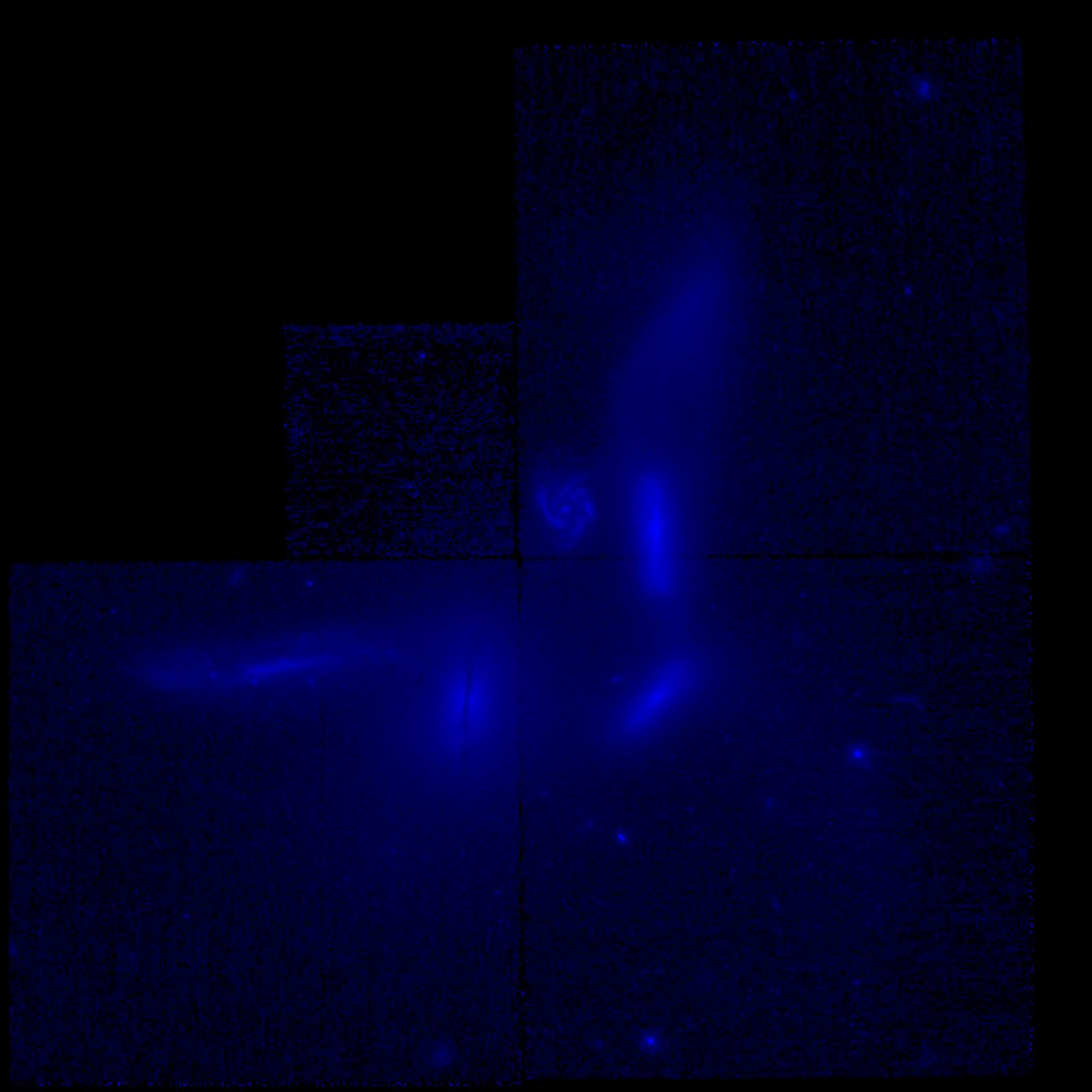Visual
Infrared

Stage 3: Combine the Layers

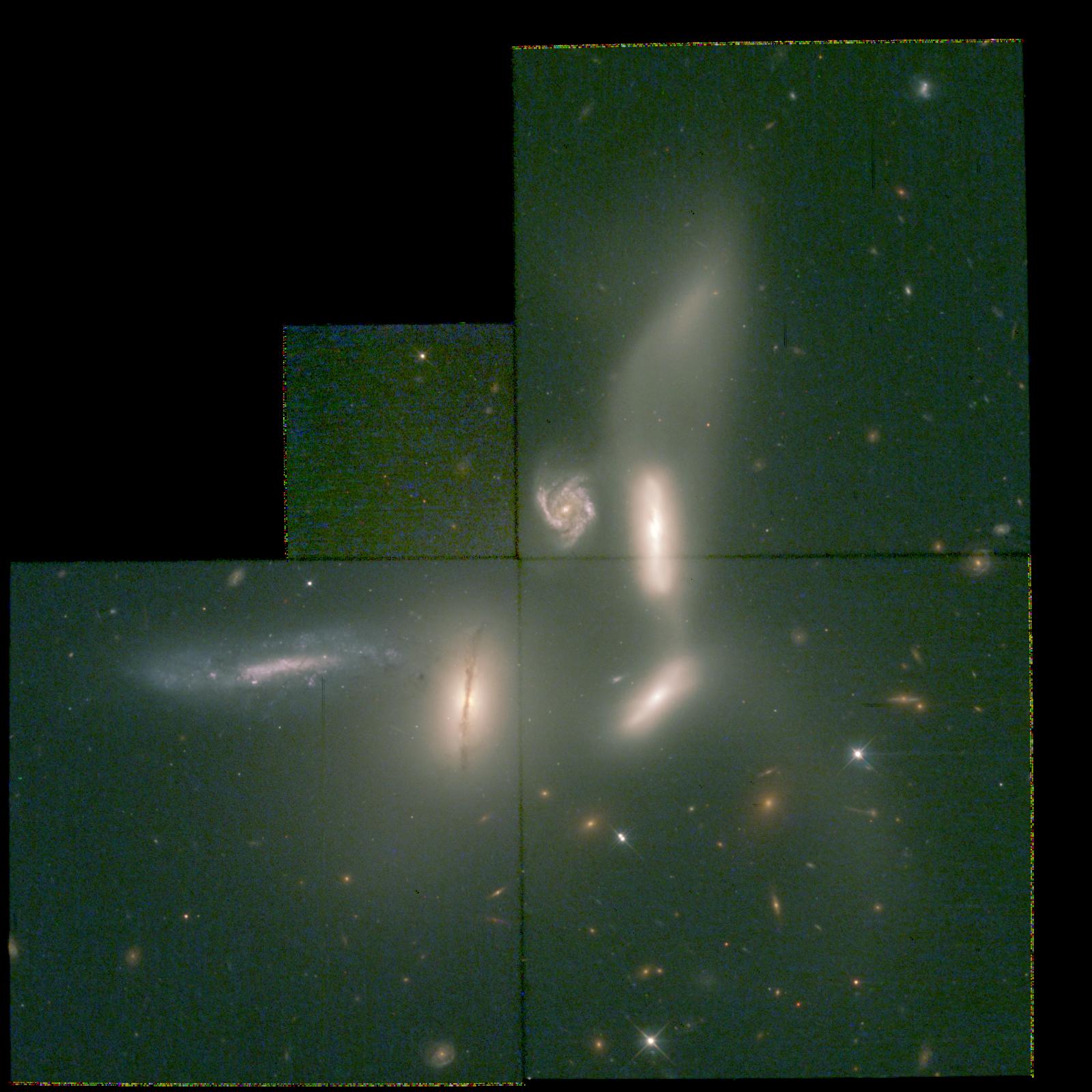
After you are satisfied in general with your colour selection, and have saved it as an .xcf file, then you flatten the image, using the Layers dialog box options, into a single tiff file with a different name in tif format.

Even better, open a new image (with a black background), Edit --> Copy Visible the display of your .xcf file and then Edit --> Paste into the new image. Set mode to screen and flatten the new image and save as a single tiff file. To flatten you use the submenus under Layers. Layers --> Merge Visible and then Layers --> Flatten.

Stage 4: Remove the Cosmetic Defects.

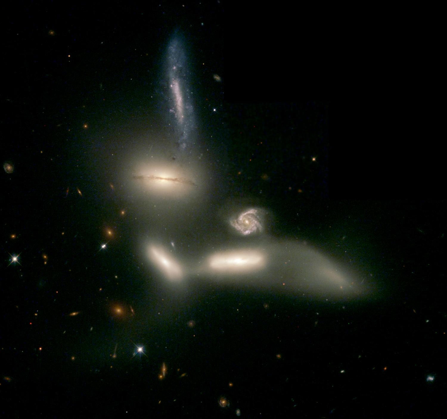
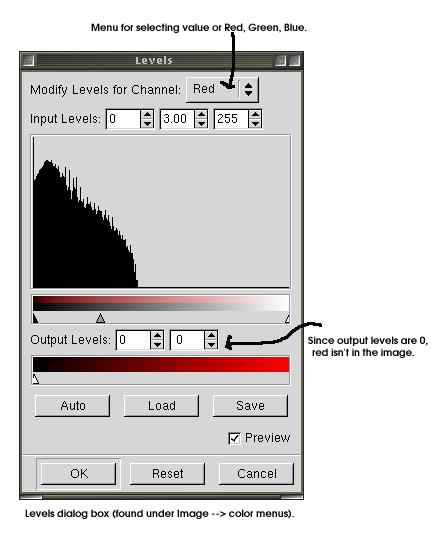
Use the image manipulation tool options (like levels) for final colour and contrast adjustments. Use the clone tool to remove chip seams and cosmic rays. Chose your orientation.

Save this file as a tiff (no compression) or, in a pinch, a 100% quality jpeg.

Back to Table of Contents