Selection of
ThAr lines for wavelength calibration of VLT/UVES
Below is a description of how I've selected ThAr lines from the
original literature line-lists in order to produce a better wavelength
calibration of UVES. However, the algorithms can easily be applied to
other spectrographs. If you'd like me to produce a catalogue for your
spectrograph of interest then "all" I need is a ThAr spectrum from
that spectrograph (covering your wavelength range of
interest).
0. Paper
A paper describing the selection procedure and results has been
accepted by MNRAS. A copy of the most up-to-date version is on astro-ph. If you use any information or results from
this paper or this web page, including the final ThAr line-list, I
would appreciate you citing the paper. The current bibliographic
information can be found on my publications page.
1. Here's all
the important data files and spectra
- The main table from Lovis et al. (2007, A&A, accepted, astro-ph/0703412): LovisC_06.dat. The first column is the vacuum
wavelength as determined by Lovis et al., the second column is the
wavelength as quoted by Palmer & Engleman (1983), the third column is
the uncertainty in the new vacuum wavelength, the fourth column is the
indentification of the line from Palmer & Engleman (1983) and the
fifth column is the intensity of the line in the HARPS spectra of
Lovis et al.
- The main table from Palmer B.A. & Engleman R., 1983, Atlas of the
Thorium Spectrum, Los Alamos National Laboratory, Los Alamos: PalmerB_83a.dat. The first three columns
are air wavelength (Angstroms), wavenumber (cm-1) and
intensity (arbitrary units).
- Table 1 from Whaling et al., 1995,
J. Quant. Spectrosc. Radiat. Transfer, 53, 1: WhalingW_95a_Tab1.dat. Format is
explained in file.
- Table 1 from Whaling et al., 2002,
J. Res. Natl. Inst. Stand. Technol., 107, 149: WhalingW_02a_ArI.dat. Format is the
same as the 1995 Whaling et al. list.
- ArI lines from Norlen G., 1973, Physica Scripta, 8, 249, between
vacuum wavelengths of 3000.0 and 11000.0 Angstroms: NorlenG_73a_ArI_v3000-v11000.dat. The
first column is Norlen's wavenumber (in cm-1) while the
second and third columns are the Norlen values increased by a factor
of [1 + 6.8x10cm-8] (see text below) given to different
precisions.
- ArII lines from Norlen G., 1973, Physica Scripta, 8, 249, between
vacuum wavelengths of 3000.0 and 11000.0 Angstroms: NorlenG_73a_ArII_v3000-v11000.dat.
Same format as for the ArI lines.
- Synthesis of Lovis et al., Palmer & Engleman, Whaling et al. and
Norlen atlases: LovisC+PalmerB+WhalingW+NorlenG_v3000-v11000.dat. See
text below for full description. This is used as the input list to the
line selection procedure.
- The final ThAr line list: thar_MM201006.dat. See text for full
description.
- The final TFITS file to be used with the UVES pipeline: thar_MM201006.tfits. This replaces
the thargood2.tfits file provided with the UVES pipeline.
- Final UVES ThAr spectrum: FITS format thar_spec_MM201006.fits and ASCII
format thar_spec_MM201006.dat.
I wrote the text below before I wrote the paper. Although the latter is more detailed and has
been refereed, the following text might still be helpful as a quick
reference or because the links might point you more directly to the
file above that you're most interested in. The text below will also be
updated in future if and when anything changes.
2. Synthesis of
existing Th and Ar line-lists
Before selecting which ThAr lines are to be used to calibrate UVES, we
first require a list of the absolute laboratory wavelengths for as
many features appearing in the UVES ThAr lamp spectrum as
possible. Most features, especially below 6000 Angstroms, are either
known to be due to Th or are unidentified (but probably due to Th),
while ~10% of the features are from Ar and <1% are from "contaminant"
species such as MgI, CaII, NaI, FeI etc. The Th and Ar lines and even
some of the contaminant lines are catalogued in various atlases
derived from painstaking (but usually rather old) laboratory
work. These atlases provide our starting point. However, every ThAr
lamp gives a somewhat different spectrum and there are always
additional lines which cannot be found in any atlas, even as
"unidentified" lines. These are probably due to additional contaminant
ions and molecular species in the lamp. This means that our knowledge
of the ThAr spectrum from any given lamp is, at best, incomplete and
this necessitates the selection procedure detailed in the next
section.
There is no single atlas of the ThAr spectrum covering the whole
wavelength range of UVES (~3030-10540 Angstroms). However, there is
one atlas of Th lines only which does cover this range, Palmer &
Engleman (1983; hereafter PE83). The PE83 absolute velocity precision
varies from about 15 to 120 m/s depending on the line intensity. PE83
identify a large number of ThI, II and III lines in their spectrum but
there is left a large number of unidentified lines which are probably
due to Th. Furthermore, on comparison with real ThAr lamp
spectra, one notices that there are still several thousand lines which
cannot be accounted for by Ar or contaminant species.
Very recently, Lovis et al. (2007, in preparation; hereafter L07) used
a large library of spectra from the highly stable HARPS spectrograph
on the 3.6-m ESO telescope to improve the situation, at least over the
wavelength range 3780-6915 Angstroms. They identified in their spectra
lines from the PE83 list which showed no positional variations with
time and obtained line positions to within an RMS of about 5-10
m/s. Thus, while bootstrapping their overall wavelength scale to that
of PE83, they were able to correct the wavelengths of individual PE83
lines, especially weaker lines, due to their large statistical
gain. Moreover, they were able to measure the wavelengths of ALL other
features in their ThAr spectra, again at the ~5-10 m/s precision
level. They removed from their list lines which saturated their CCD,
(very few) lines which appeared in the PE83 catalogue but which were
too weak for them to detect and, most importantly, they removed lines
which were either closely blended with other lines or were observed to
change position with time. The latter indicates either that the line
experiences significant shifts with changing lamp pressure or current
or that the line is actually a blend and that the relative intensities
of the blended lines vary with changing lamp conditions.
The L07 catalogue ranges from 3780 to 6915 Angstroms. Thus, the PE83
line list is used for Th and contaminant lines outside this
range. However, to ensure that the maximum number of lines are used to
calibrate UVES and to properly select which lines are most useful
(i.e. to reject blends) it is desirable to use the known Ar lines as
well. Three useful Ar line-lists exist - Norlen (1973; hereafter N73),
Whaling et al. (1995; hereafter W95) and Whaling (2002; hereafter W02)
- each of which has different advantages and disadvantages. N73
contains both ArI and ArII whereas W95 contains ArII lines and W02
contains ArI lines. The sensitivity of the N73 experiment was worse
than W95 and W02 and so fewer lines are listed. The velocity precision
achieved by N73 for the ArI lines is better than that of W02 but the
ArII lines of W95 should be more precise than N73's. Finally, there is
a calibration difference such that the Whaling wavenumbers
are larger than the Norlen ones by a factor of SNW =
[1 + 6.8x10^{-8}]. Whaling's calibration should be more reliable and
so we choose to use the Whaling calibration scale in synthesising the
Argon line-lists.
The different lists of ArI and ArII lines are combined in the
following ways. We do not consider the ArIII lines from W95 since
there are very few of them and since their wavelengths tend to be
sensitive to the pressure and current in the ThAr lamp.
- ArI: W02 recommends using the Norlen wavenumbers (scaled by
SNW). So N73 values (with scaling) were used when
available, otherwise W02 values were used. For N73 values, the
intensity scale of N73 was used as re-cast by De Cuyper & Hensberge
(1998) onto a log10 scale. For W02 values, the W02 intensity scale was
used.
- ArII: W95 values were used here since W95 claims there is no
strong dependence on pressure and their values are more precise than
N73's. In the few cases where N73 reports an ArII line that W95
doesn't, the N73 value (scaled by SNW) is used. For
W95 lines the W95 intensity scale (which is the same as the W02
intensity scale) is used. For N73 values, the intensity scale of N73
was used as re-cast by De Cuyper & Hensberge (1998) onto a log10
scale. Note that N73 uses the intensity scale of Minnhagen (1963) for
ArII lines above lambdaair=7600A and below
lambdaair=3400A. This subtlety is neglected in the
considerations below.
After combining the L07, PE83, N73, W95 and W02 lists in the above way
we obtain the file LovisC+PalmerB+WhalingW+NorlenG_v3000-v11000.dat,
hereafter referred to as LPWN. The format of the file is the same as
that of the final ThAr line list which is described in Section 4. One
difference is the intensity measures reported. Note from the above
that the intensity scales for each species (e.g. ThI, ArI, ArII) are
different and that the relative intensities of lines from different
species depend on many factors, such as lamp pressure and current and
the relative partial pressures of Th and Ar gas used. In LPWN we keep
the original intensity measures described above.
3. ThAr line
selection
One should not simply use the above line-list, LPWN, to calibrate UVES
spectra because of the potential for line-blending. The FTS spectra of
PE83, N73, W95 and W02 and the HARPS spectra of L07 all have resolving
powers R >= 120,000 whereas the UVES resolving power is typically
35,000-70,000 and possibly as high as 110,000. Therefore, a major part
of the line-selection that follows is the rejection of "close"
blends. The concept of "close" clearly depends on the relative
intensities of the blended lines and so it is necessary to put all
lines in the above list onto the one intensity scale typical of
measured UVES ThAr spectra. Furthermore, since there are always
additional unknown lines in measured ThAr spectra, a given ThAr line
can only be used for calibration if it is measured to be
reliable in the UVES ThAr spectrum. For these reasons we have
constructed a UVES ThAr spectrum for use in the line selection
process.
3.1 UVES ThAr
spectrum
ThAr spectra taken with a 0.6 arcsecond slit and no CCD rebinning were
retrieved from the ESO VLT archive. Several exposures were used, each
taken in a different standard UVES wavelength setting (346, 437, 580,
600, 760 and 860nm) so that complete wavelength coverage was achieved,
with the exception of three small echelle order gaps redwards of
1000nm (1008.443-1008.593nm, 1025.242-1025.695nm &
1042.610-1043.376nm). The UVES pipeline was used to extract and
wavelength calibrate the data. Several modifications to the pipeline,
described here, were made to
improve object extraction and wavelength calibration. The data were
re-dispersed to a log-linear wavelength scale using UVES_popler, code specifically written to
re-disperse and combine multiple wavelength setting data from
UVES. Overlapping regions of spectra were cut away so that only one
raw exposure contributed to the final spectrum over echelle-order
scales. No effort was made to flux calibrate the final spectrum and
the blaze-function of the echelle grating was still evident in the
data. However, our results from the intensity re-scaling in the next
section demonstrate that this is a minor consideration. The final
spectrum has a resolving power of R ~ 70,000 and the log-linear
dispersion is set to 1.75 km/s.
3.2 ThAr selection
algorithm
The above line-list, LPWN, is treated as the input catalogue to the
following algorithm for selecting a final list for calibration of
UVES. We make three passes through the algorithm, altering the line
list used to calibrate the UVES ThAr spectrum and other parameters
specified below. All plots below pertain to the final pass through the
algorithm.
- UVES ThAr spectrum calibration: The above procedure for
constructing the UVES ThAr spectrum requires an input line-list for
the wavelength calibration stage. At the first pass we use the
line-list provided by ESO with the UVES pipeline (thargood_2.tfits, pipeline_thar.dat). At the second and
third passes the output from the previous pass through the algorithm
is used.
- Gaussian fitting: Each line in the input list LPWN is
searched for and fitted with a Gaussian. The fit includes the 13
pixels centred on the pixel with maximum intensity. A first-guess
continuum is defined by averaging the first and last 2 pixels in the
window. A first-guess continuum slope is defined by taking the
difference between the average of the last 2 and first two pixels. A
first-guess intensity is defined as the maximum intensity minus the
continuum level. A first-guess width is defined by taking the velocity
difference between the first and last pixels which have intensities
below the continuum plus half the first-guess intensity. The
first-guess central velocity is calculated as the intensity weighted
velocity of the 3 central pixels. A 5-parameter Gaussian fit is
performed and the best-fit parameters used in subsequent steps. The
initial guesses and Gaussian fitting procedure is identical to that
used in the UVES pipeline (see modifications made to pipeline).
- Intensity re-scaling: The different Th and Ar atlases
combined above have different intensity scales. Furthermore, one
would not expect to find the same relative intensities for lines of
different ionic species (e.g. ArI and ArII) in the laboratory and
astronomical spectra since the ThAr lamps used will have had different
operating conditions (e.g. pressure, current etc.). We therefore aim
to place all lines from the different ionic species (ThI, II & II, ArI
& II, XX 0 & 1) from each different intensity scale ("L", "P", "N" &
"W") on a single intensity scale directly related to the UVES ThAr
spectrum. First, any pairs of lines within 13 km/s of each other are
removed from the input line list LPWN. For each category of line -
that is, one of "ThI L", "ThI P", "ThII L", "ThII P", "ThIII L",
"ThIII P", "ArI L", "ArI N", "ArI W", "ArII L", "ArII N", "ArII W",
"XX 0 L", "XX 0 P" or "XX 1 L" - the median ratio of the measured and
expected intensities of remaining lines, alpha, is defined as the
scale-factor. All lines from this category are then scaled to the UVES
intensity scale by multiplying their listed intensities by alpha. Two
examples of this process are shown in Fig. 1. Figure 2 shows all lines
from all categories placed on the UVES intensity scale.
Figure 1: Examples of the intensity scaling procedure. Measured
and expected intensities for unblended lines from each category
(e.g. "ThI L", "ThI P") are compared to derive the scale-factor,
alpha. All lines from that category are then scaled to the UVES
intensity scale using alpha.
Figure 2: Lines from all categories placed on the UVES
intensity scale. The red points are lines from the initial list which
satisfy the blending criteria defined in step 4 of the ThAr selection
algorithm. The black points are lines satisfying all selection
criteria and constitute the final ThAr line-list. Here,
Ilist refers to the re-scaled listed
intensities.
- Blend removal: If, when Gaussian-fitting a single line,
another weaker blending line is present but ignored in the fit then
the centroid returned from the fit will be shifted towards the
blending line. The magnitude of the shift will depend not only on the
velocity separation between the two lines, dvsep,
but also on the relative intensities of the two lines,
I2/I1. When the two lines are not
resolved from one another, it is easy to approximate the velocity
shift. The new centroid wavelength can be approximated by the
intensity weighted mean wavelength of the two blended lines,
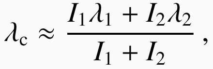
and so the velocity shift due to the blending line is
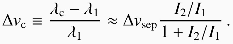
However, if the two lines are further apart and are partially
resolved, it is not clear how dvc will depend on
dvsep and
I2/I1. Figure 3 (right) shows the results
of a numerical experiment where two blended lines are varied in
relative intensity and separation and fitted with a single Gaussian
with similar initial guesses as in step 2. A by-eye fit to the
contours of constant velocity shift gives the following
relationship:
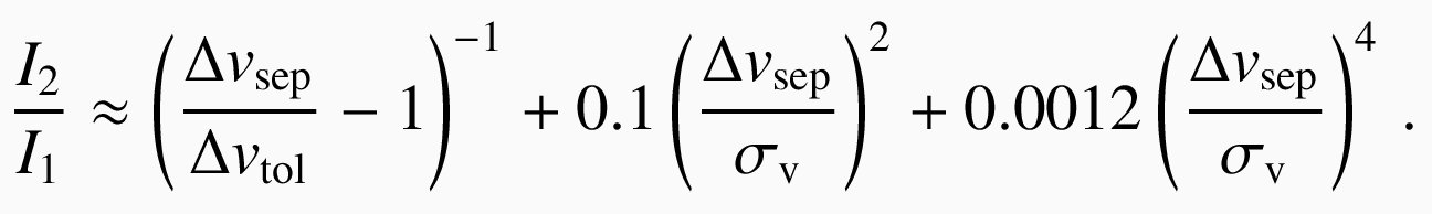
The first term on the right-hand-side is just the previous equation
and applies when dvsep is small with respect to
sigmav = FWHM/2.355. We therefore reject lines from the
input line-list LPWN which have blending lines within 13 km/s with
relative intensities greater than that predicted by the above equation
to produce shifts greater than a tolerance of 40 m/s. This tolerance
is roughly equal to the overall wavelength calibration residuals
achievable with the UVES pipeline using the final ThAr list.

Figure 3: Removal of strongly blended lines from the
list. Right/Bottom: The shift in the centroid of a synthetic
Gaussian due to blending with a weaker line. Both lines have widths
typical of those seen in our UVES ThAr spectrum. The black dashed
lines are contours equally spaced in the logarithm of the shift. The
solid red line is a simple "fit" to these contours at a velocity
tolerance of 40 m/s (see above equations). All lines with weaker lines
more than 13 km/s away are safe from velocity shifts greater than ~40
m/s and this is marked with the vertical dashed red
line. Left/Top: Pairs of lines in the input line-list LPWN with
the same solid red line from the right-hand panel.
- Removal of weak lines: If ThAr lines appear weak in the
UVES lamp spectrum then the UVES pipeline's line-identification
algorithm can fail or yield a false identification. The amount of
velocity information in weak lines is also too small to be useful in
calibrating the wavelength scale of UVES. We therefore reject any
lines with measured intensities (above the measured continuum) less
than 4 times the measured continuum level.
- FWHM selection: Any additional unknown features in the UVES
ThAr spectrum can cause blending with the remaining lines from the two
selection steps above. The next three steps aim to reject those lines
which are effected in this way. The first of these steps is to remove
lines whose widths are clearly inconsistent with the instrumental
resolution, in this case R ~ 70,000 or FWHM ~ 4.3 km/s. Figure 4 shows
the distribution of FWHM for all lines surviving the previous two
selection steps. After visual inspection of the lines lying away from
the main cluster around FWHM ~ 4.3 km/s it was clear that lines wider
than ~ 5.3 km/s and narrower than ~ 3.5 km/s should be removed. Lines
were fitted as too wide when blended with other unknown features or
where saturation of the CCD occurred. Lines were fitted as too narrow
usually when they were very weak.
Figure 4: The FWHM distribution of the lines surviving the
previous selection steps. The structure seen in the main congregation
of points is due to slightly differing resolutions in the different
exposures from different wavelength settings.
- High slope rejection: One of the improvements made to the UVES
pipeline was the addition of a continuum slope parameter to the
Gaussian fitting of ThAr lines during the wavelength calibration. If a
line is close to a strong, previously unknown feature in the UVES ThAr
spectrum then a large slope (relative to the line's intensity) might
be needed to fit the line properly. Since these unknown features
probably vary with lamp conditions, one might regard lines fitted with
large continuum slopes as best avoided when calibrating the wavelength
scale of UVES. Figure 5 shows the distribution of the absolute velocity
difference, dvs, between two Gaussian fits - one made
including the slope parameter, the other made with the slope fixed to
zero - with continuum slope normalised by the line intensity. Visual
inspection of lines with dvs greater than 80 m/s
showed that some of them have large asymmetries which are probably due
to close blends with unknown features. Therefore, all lines with
dvs >= 80 m/s are rejected.
Figure 5: Distribution of the absolute velocity difference
between the centroids of two Gaussian fits - one made including the
slope parameter, the other made with the slope fixed to zero - with
the continuum slope. A conservative cut is made at
dvs = 80 m/s to reject lines which might be effected
by additional unknown features in the UVES ThAr spectrum.
- Large residual rejection: As a final selection step we
reject lines surviving all previous selection steps which are fitted
at wavelengths at some variance with those expected from the input
line list LPWN. In the first pass through the selection algorithm we
do not apply this criterion because of possible inaccuracies in the
ThAr line-list supplied with the UVES pipeline. In the second pass we
reject lines which are fitted at positions more than 0.25 km/s away
from the expected position. In the third pass we reduce this parameter
to 0.15 km/s.
4. Results
The ThAr line-list formed after the third pass through the selection
algorithm, referred to as the final list, is available as an ASCII
file, thar_MM201006.dat, and as a
TFITS file suitable for use with the UVES pipeline, thar_MM201006.tfits. The latter has
some additional lines added from LPWN at the beginning and end of the
file to satisfy some requirements of the UVES pipeline. However, these
lines are not used in the calibration. The TFITS file should replace
the thargood_2.tfits file provided with
the UVES pipeline.
The first column of thar_MM201006.dat
is the wavenumber, omegai, in cm-1
[lambdavac = 1x10⁸/omegai] for
each line, i. The second column is the air-wavelength computed
from lambdavac using the Edlen (1966) formula for the
dispersion of air at 15 degrees C and atmospheric pressure (see Murphy
et al. 2001 for detailed discussion). The third column is the
logarithm (base 10) of the original listed intensity scaled to the
intensity scale of the UVES ThAr spectrum (described above). The
fourth and fifth columns provide the line identification when
available. If the line is unidentified then "XX" is used as the
element designation and an ionization level of either "0" or "1" is
given. The final column identifies the source of the wavenumber and
which intensity scale the line was originally on: "L" indicates L07,
"P" indicates PE83, "N" indicates N73 while "W" indicates W95 or
W02. For "XX" lines in L07 the ionization is given as "0" if the
unidentified line appears in PE83 and as "1" if L07 claim the line was
previously unknown.
The initial input list LPWN contains 13903 lines while the final list
contains just 3070. For comparison, the line-list supplied with the
UVES pipeline contains 2387 lines over the wavelength range covered by
UVES. So, although a large number of lines are rejected in the
selection algorithm, there are certainly enough remaining lines to
provide a reliable calibration of the UVES wavelength scale. Figure 6
(left) shows the distribution of lines with wavelength in bins which
approximate the size of extracted UVES echelle orders. Compared to the
initial input list, the distribution of lines is quite uniform. This
is mainly because of the rejection of close blends. Note also that
there are always more than ~20 useful lines per UVES echelle order in
the final list. This is enough to supply a reliable and accurate
wavelength calibration solution. Figure 6 (right) shows the
distribution of lines at each step of the third pass through the
selection algorithm. None of the steps after the rejection of blends
removes lines in a strongly wavelength-dependent manner, as
expected. Figure 7 (left) shows the contribution from Th, Ar and
unidentified lines in the initial input list LPWN and Fig. 7 (right)
shows the composition of the final list. One notices the strong
decrease in the fraction of unidentified lines through the selection
algorithm. This is because most of the unidentified lines are those
newly discovered by L07, many of which are quite weak and/or blended
at the UVES resolution.

Figure 6: Histograms showing the expected number of lines per
echelle order for different line-lists. Left/Top: Comparison of
the initial line-list with the list after close blends have been
removed. Also a comparison of the final line-list with that provided
with the UVES pipeline. Right/Bottom: The reduction of the
line-list through the various selection stages.
Figure 7: Histograms showing the contributions from Th, Ar and
unidentified lines to the initial (left/top) and final (right/bottom)
ThAr line-lists.
We have used the final list to calibrate the UVES ThAr spectrum a
final time and the resulting spectrum is available as a FITS file, thar_spec_MM201006.fits, and an
ASCII file thar_spec_MM201006.dat. The former
is readable with IRAF and the formats of both files are fully
explained in the documentation for UVES_popler. In extracting and
wavelength calibrating the spectrum with the UVES pipeline, we noted
an improvement in the wavelength calibration residuals of more than a
factor of 3: Using the version of the UVES pipeline distributed by ESO
(i.e. without the modifications described here) and the line-list provided
with the UVES pipeline, wavelength calibration residuals of about 140
m/s were acheived for the unbinned ThAr frames discuss above. In our
final calibration using the final ThAr line-list, we achieved
wavelength calibration residuals 40 m/s over the entire wavelength
range without losing too many lines; an average of >=15 lines were
utilized per echelle order by the wavelength calibration
software.
To demonstrate the strong advantage of using the new line-list (thar_MM201006.dat, thar_MM201006.tfits) in preference to
the one distributed by ESO with the UVES pipeline (thargood_2.tfits, pipeline_thar.dat), we have also reduced
the same raw ThAr exposures used above with the unmodified UVES
pipeline and the thargood_2.tfits
line-list. We use the new line-list to trace any distortions of the
wavelength scale and the results are plotted in Fig. 8. The ThAr lines
in the spectrum are fitted in the same manner as described above
(Section 3.2, step 2) and the residual between the fitted wavelength
and the wavelength listed in thar_MM201006.dat is calculated. The mean
of the residuals shows strong, statistically significant variations
with wavelength. For example, the difference between the mean residual
at 6000 and 6300 Angstroems is about 75m/s!
Figure 8: Distortions of the wavelength scale introduced by the
ESO UVES pipeline and ThAr line-list. A ThAr spectrum was reduced
using the original UVES pipeline, without modifications, and its
accompanying line-list and the ThAr lines are fitted with
Gaussians. The residual between the fitted wavelengths and those
expected based on our final line-list, thar_MM201006.dat are plotted versus the
wavelength. The structure in the residuals is traced by the green line
which is calculated by taking the mean in bins which cover
approximately two echelle orders.
References
Edlen B., 1966, Metrologia, 2, 71
Palmer B.A., Engleman R., 1983, Atlas of the Thorium Spectrum, Sinoradzky H. (ed.), Los Alamos National Laboratory
Lovis et al., 2007, A&A, accepted, astro-ph/0703412
Minnhagen L., 1973, J. Opt. Soc. Am., 63, 1185
Murphy M. T., Webb J. K., Flambaum V. V., Churchill C. W., Prochaska J. X., 2001, Mon. Not. Roy. Soc., 327, 1223
Norlen G., 1973, Physica Scripta, 8, 249
Whaling et al., 1995, J. Quant. Spectrosc. Radiat. Transfer, 53, 1
Whaling et al., 2002, J. Res. Natl. Inst. Stand. Technol., 107, 149
De Cuyper J.-P., Hensberge H., 1998, Astron. Astrophys. Supp. Ser., 128, 409
Last updated: 20th October, 2006 by Michael Murphy